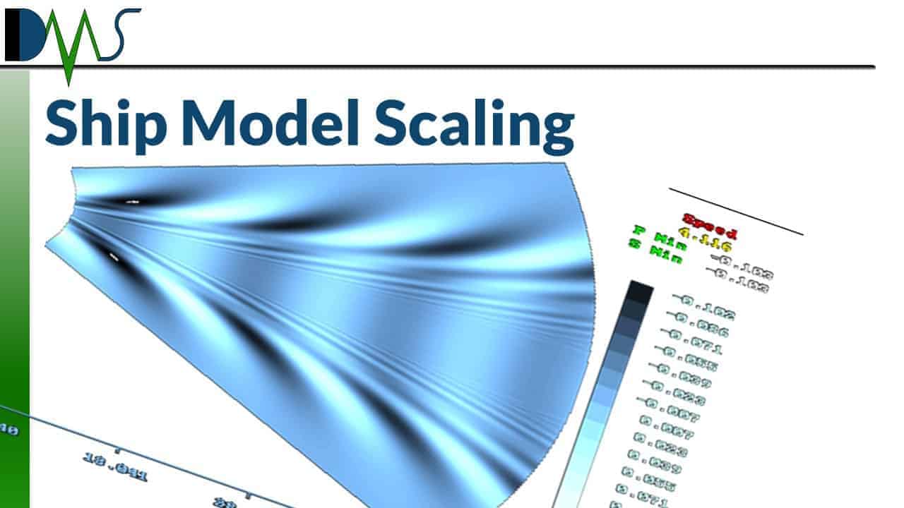
Ship Model Scaling

1.0 Introduction

What good are model
experiments, we want big ships! Model
experiments only help if we can match those measurements to equivalent values
at the full ship scale. Easier said than
done. We developed a whole new field of
fluid mechanics just to answer this challenge.
This is where the science of modern ship design began: how to reliably convert from model scale to
ship scale.

2.0 Two Important Forces

The issues around model scaling arise because we need to
scale two different forces. Ship
resistance developed from two major forces:
viscous and waves. Viscous forces
are basically skin friction, plus some flow interactions at the stern of the
ship. The second category of forces come
from waves. These generate primarily at
the bow and the stern, creating fascinating wave patterns that change with
speed. (Figure
2‑1)

Most importantly, these two
forces behave very differently. Table 2‑1 summarizes the major differences between these two forces. (Table
2‑1 references some terms explained later in this article.) We employ entirely different rulebooks for
them. Different math, different physics,
and different formulas to convert them from model scale to ship scale.

Viscous Forces	Wave Forces
Tied to fluid viscosity	Tied to gravity
Force coefficient reduces with increased speed	Force coefficient increases with increased speed
Reynolds number dependent	Froude number dependent
Dominates at low speeds	Dominates at high speeds

Table 2-1: Comparison of Ship Resistance Forces

3.0 Non-Dimensional Numbers

Model scaling and experimental analysis are about more than just raw numbers. We seek understanding, discernible patterns, predictable behaviors. That is why naval architects usually examine resistance with another tool: non-dimensional coefficients. Non-dimensional coefficients are math formulas, used to reformat experimental data. They take the raw force of resistance and factor out ship size and speed. (This works at both model scale and ship scale.) Reformatting the data into these coefficients clarifies patterns and allows us to make meaningful comparisons between different ships.

For example, Figure 2‑1
plots raw resistance forces for a typical ship.
It’s difficult to identify significant patterns in this graph. When reviewing data, naval architects want
simple graphs so they can isolate cause and effect of any changes in our
designs.

This time, Figure 2‑2
plots the same forces, formatted as resistance coefficients. The patterns are much easier to identify and
better segmented. For example, the blue
line of the wave coefficient clearly shows three distinct regions:

A rising slope from 0 to 1.0 m/s
A region with an oscillating pattern from 1.0 to
about 2.5 m/s
A region where the slope rapidly increases to a
new plateau from 2.5 to 4.25 m/s

That graph clearly demonstrates regions of significant
changes. Resistance coefficients make
the patterns easier to identify. And
they allow us to compare between different ships.

3.1 Model Scale Conversions

Resistance coefficients also work for the same ship at
different scales. This allows us to
convert from model scale to full scale.
Under the right speed conditions, we use resistance coefficients to
scale up the results, following this process:

Record experimental forces from model scale
Convert model scale forces into resistance
coefficients by factoring out the model size and speed.
Apply the size and speed of the full scale ship
to get the full scale results.

Unfortunately, the process is far more complicated. I said that simple resistance coefficients
work under the correct speed conditions.
But physics makes it impossible to find the correct speed, thanks to
something called the scaling correlation problem.

4.0 The Scaling Correlation Problem

The scaling correlation problem depends on selecting the
correct speed, and there are formulas that match model speed to ship
speed. These formulas are more
non-dimensional coefficients.

Resistance coefficients worked for forces; so we also have
non-dimensional coefficients for speed.
These speed coefficients depend on the ratios of the dominant fluid
physics in play, and we use different formulas for different situations, with
each formula generally named after the person who first developed it. For example, a submerged submarine would use
the Reynolds Number as a coefficient for speed.
Reynolds Number focuses on the ratio between the momentum of the water
and its viscosity. (The actual math is a
little more complicated than a simple ratio.)

The fathers of fluid dynamics derived several different
coefficients, based on different combinations of dominant forces. William Froude was famous for the Froude
Number, which centered around the relation between gravity and momentum of
water. The Froude Number was particularly
important to characterize waves.

These speed coefficients tied into that issue of finding the
right speed conditions. To convert from
model scale to ship scale, you need to match the speed coefficient at both scales. This ensures the correct balance between the
dominant forces at both scales, allowing you to correctly apply the force
coefficients.

And this is the crux of the scaling correlation
problem. Ship resistance is dominated by
two major forces: waves and viscous
resistance. That correlates to two
different speed coefficients: the Froude
Number and the Reynolds Number. Two
different formulas that work in opposite directions. Figure 4‑1
compares these two coefficients for different model scale factors, at a single model
speed. In theory, we could achieve the
correct speed for perfect scaling correlation at the point where these two
lines intersect.

That theory has several practical limitations. First, the intersection point changes with
each speed. To achieve perfect
correlation, we would need to construct a different model for each speed that we
wanted to test. And ship models are not
cheap, making it infeasible to build 7-10 models for a single test.

Artificial gravity is also infeasible, which is what you
would need to achieve the graph in Figure 4‑1. To create the intersection that you see in
the graph, I assumed that gravity changed between model scale and ship
scale. Mathematically, this is perfectly
valid. Practically, gravity stays approximately
the same everywhere on planet Earth, at ship scale or model scale. Unless you can invent cheap artificial
gravity, the scaling correlation problem is impossible to solve.

5.0 ITTC Scaling Procedure

If we can’t solve the scaling correlation problem, we need
to get around it. The international
towing tank conference (ITTC) developed a procedure to subtract out the viscous
coefficients, so we only deal with one set of forces at a time. Now the scaling procedure goes roughly like this:

Record experimental forces from model scale
Convert model scale forces into resistance
coefficients by factoring out the model size and speed.
Subtract out the viscous coefficient using the
ITTC correlation line at model scale.
Recalculate ITTC correlation line at ship scale
to estimate viscous coefficient at ship scale.
Add in the estimated viscous coefficient at ship
scale.
Apply the size and speed of the full scale ship
to get the full scale results for the ship.

(Actually, the ITTC scaling procedure is more
complicated. But this articles only
focuses on the major concepts of the procedure.)

5.1 ITTC Correlation Line

The ITTC correlation line was the key to solving the scaling
correlation problem. The idea for the
correlation line started with William Froude.
He towed flat plates down a tank to discover a simple formula for estimating
the viscous coefficient. (Figure
5‑1) Over the years, we improved on the work of
William Froude to develop a formula that very closely estimates the resistance
coefficient.

Figure 5‑1: Flat Plate Tests [1]

The key behind the ITTC correlation line is the uniform application. This formula provides a very good estimate, but not perfect. Thankfully, that doesn’t matter. Every towing tank in the world uses the same formula. Even though the formula has imperfections, every tank works with the same issues. Each tank adds on a small safety factor to correct for these imperfections, plus other complications of scaling that I have not covered. This works specifically because every tank uses the same baseline procedure as their starting point, and any additional corrections are small. Go to any decent tank in the world, and you will get nearly the same process. That consistency was the key to scaling model test results up ship scale values.

6.0 Conclusion

Sadly, physics makes it impossible to perfectly scale model
test results up to ship scale. But we
found a way around the scaling correlation problem. The beauty of the ITTC correlation line was
recognizing practical engineering. We
don’t need to be perfect, just close and consistent. Add in a small safety margin, and you have a
reliable method to scale from model scale to ship scale.

7.0 References

[1]	YouTube Creator, “Towing a Flat Plate,” YouTube, 26 Feb 2009. . Available: https://www.youtube.com/watch?v=G5slCVPAN1s. .
[2]	A. F. Molland, S. R. Turnock and A. D. Hudson, Ship Resistance and Propulsion, 2nd edition, Cambridge, UK: Cambridge University Press, 2017.

1.0 Introduction

2.0 Two Important Forces

3.0 Non-Dimensional Numbers

3.1 Model Scale Conversions

4.0 The Scaling Correlation Problem

5.0 ITTC Scaling Procedure

5.1 ITTC Correlation Line

6.0 Conclusion

7.0 References

Share This Post

More Like This

Surviving the Arctic: Polar Class Icebreakers

Ramming the Ice: Icebreaker Propulsion

Breaking the Ice: Icebreakers

Lying with Numbers

The Value of Life

How Propulsion Works: Classifying Ship Propulsion

Stability Letters Explained

Class Societies

5 Steps to (NOT) Build a Boat

Our Socials

About Us

What We Do

Contact Us