Stability Test Theory

What science could possibly link moving a few weights on deck with calculating the light ship weight? Armed with knowledge, we carefully exploit physics to achieve high quality science without the fancy equipment. Today I explain some of the theory behind the stability test.

The Math Behind The Measurements

1.0 Introduction

After you complete the stability test, we break out the black magic.  Once the stars align, we consult the oracle and interpret the portents to convert the test data into the light ship. . . .

Clearly, the actual math involves a far more mundane process.  But it does make you wonder.  What science could possibly link moving a few weights on deck with calculating the light ship weight?  Today I explain some of the theory behind the stability test.

1.1 Disclaimer

This article provides the broad overview of the calculations and theory for a stability test.  But I don’t show the full mathematics, partly to protect DMS competitive advantage. 

2.0 Goal

We want to calculate four critical numbers for the vessel light ship.

• Weight
• Longitudinal center of gravity (LCG)
• Transverse center of gravity (TCG)
• Vertical center of gravity (VCG)

These four numbers completely define the vessel weight properties.  First, we calculate this information for the vessel, as-inclined.  This includes the light ship, plus everything that shouldn’t be there.  And then we correct for the extra items like deadweight, test equipment, people on-board, etc.

3.0 Stability Model

 In the old days, any stability calculations required hand calculations and integrations along the lines plan, using Bonjean curves and Simpson’s Rule integration.  They were terribly cumbersome and laborious. 

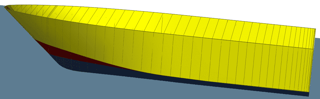
 Thanks to computer technology, we have a better method.  We construct a 3D stability model from the lines plan. (Figure 2‑1)  This contains a 3D definition of the hull shape, defined in the stability analysis software.  The software performs those same integrations, but infinitely faster.  Once the computations became faster, we asked for better resolution and better accuracy.  Computers delivered.  The modern stability model is far superior to hand calculations in every respect.  Stability models have become an essential tool for the modern stability test.

 As mentioned, the stability model follows the same basic principles as the original Bonjean curves.  The stability model defines the hull as a series of transverse sections (many sections).  We then define a waterplane for the hull, and the stability model translates that into a water level definition for each individual section.  With this knowledge, the stability model calculates the submerged area at each transverse section.  Combine that with a knowledge of the spacing and location for all sections, and the stability model instantly calculates a host of information about the vessel buoyant properties for that specific waterplane.  

4.0 Weight, LCG, TCG

 The weight, LCG, and TCG come from the freeboard measurements.  We use the freeboard measurements and the vessel drawings to calculate the draft at several locations along the vessel length.  Based on those drafts, we simultaneously calculate the vessel draft, trim, and heel.  This completely defines the current waterplane for the vessel.

 Once we have the current waterplane, we punch that information into the stability model (draft, trim, and heel).  This is where the stability model really saves time.  It instantly calculates the vessel hydrostatics and reports the resulting weight, longitudinal center of buoyancy (LCB), and transverse center of buoyancy (TCB) to match that waterline.  When the vessel sits in equilibrium, the LCG must equal the LCB and the TCG must equal the TCB.  As a result, the hydrostatic properties tell us weight, LCG, and TCG.

 Technically, this whole calculation is possible by just measuring three points on the ship.  But what if the measurement was wrong?  An error of even 10 mm can mean an extra 50 MT of weight for the ship.  So we need to be sure about our measurements.  That is why we take multiple freeboard measurements along the vessel length to calculate the current waterline for the vessel.

Your content goes here. Edit or remove this text inline or in the module Content settings. You can also style every aspect of this content in the module Design settings and even apply custom CSS to this text in the module Advanced settings.

5.0 Vertical Center of Gravity (VCG)

We still need one last piece of information:  the VCG.  This is also the most critical information.  Calculation of the VCG requires a two step process.  First, we calculate the GM_T.  Second, we use the GM_T to calculate the VCG.

 5.1 GM_T Calculation

GM_T starts with the metacentric height.  The metacentric height stands for an imaginary pivot point.  As the ship heels over, the center of buoyancy shifts, because the underwater shape changes. (Figure 5‑2)  If you imagine that center of buoyancy swinging like a pendulum on an imaginary string, the pivot point would be the metacenter.  And GM_T is the vertical distance from the metacenter to the VCG (shown at point G in Figure 5‑1).

So how do we determine the GM_T from the incline experiment?  I first need to talk about the physical meaning of GM_T.  Imagine the ship acting as a giant spring.  As you heel it over, the heeling moment slowly increases.  If the ship were a spring, the GM_T would be our measure for the strength of that spring, called the spring rate.

At small heel angles, this analogy matches real life.  The ship demonstrates a very predictable and linear response as it heels over.  That’s good.  Linear responses mean easily detectable patterns.  This is the goal of the incline experiment:  calculate GM_T.

GM_T comes from the relation between righting moment and heel angle.  So we need to measure those two values.  By moving weights to different transverse positions on the deck, we create a known heeling moment.  We create that heeling moment without changing the total weight of the vessel at any time.  This is fundamental to the entire stability test and underlying theory.  The vessel weight remains constant throughout the entire test.

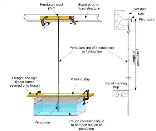
After moving the weights, the vessel heels over.  We very accurately measure the heel angle.  The most popular tool is pendulums. (Figure 5‑3)  We like pendulums because they can be constructed on-site and adapted to each situation.  Despite their simple construction, pendulums easily measure with an accuracy around 0.01 deg or smaller.

Combine the heel moment and heel angle, and you can produce a plot like Figure 5‑4, commonly called a tangent plot.  Everything builds to this tangent plot. The whole goal was to get that clear line on the tangent plot, because the slope of that line directly correlates with the GM_T.  If you know the slope of the line, you can calculate the GM_T.

5.2 VCG Calculation

After determining the GM_T, we next convert that over to the important number:  vertical center of gravity (VCG).  Fortunately, there is a simple relation between GM_T and VCG. (Equation 1)

VCG = KG + BM_T – GM_T – FSC (Equation 1)

We can determine KB and BM_T strictly from the geometry of the hull shape and the current vessel draft.  The free surface correction adjusts for any slack tanks currently in the vessel.  The incline experiment just yielded GM_T.  That provides all the missing pieces of the puzzle.  This yielded the all important value for the vertical center of gravity (VCG).

6.0 Removing Deadweight

Sections 2.0 through 5.0 created a good starting point.  We now calculated a reliable number for the current weight and center of gravity for the vessel.  However, that is not the true light ship.  The as-inclined condition includes many unwanted weights in the calculation:

Deadweight items

• Incline equipment
• Incline weights
• Tank contents

This is where the deadweight survey and tank survey come in.  Before the incline experiment, all of these items were meticulously detailed and tallied up.  We know the weight and location for all the outstanding items.  Now we apply simple weight / moment calculations to remove all those unwanted weights on paper. (Table 6‑1)

7.0 Conclusion

 Moving concrete blocks across the deck of a ship doesn’t seem very glamorous.  It certainly fails to indicate the precise nature of a stability test.  And that is what I love about stability tests.  We don’t require fancy equipment or expensive testing facilities.  All we require is a little knowledge about the ship.  Armed with knowledge, we carefully exploit physics to achieve high quality science without the fancy equipment.  Now that’s efficient.

8.0 References

Relevant Ship Science Articles